Highpass and lowpass filters
Here we look at the choice of filters both for low and high pass.
import os.path as op
import sys

import numpy as np
from scipy.signal import freqz
import matplotlib.pyplot as plt

from mne.filter import create_filter

sys.path.append(op.join('..', '..', 'processing'))
from library.config import set_matplotlib_defaults, annot_kwargs  # noqa: E402

set_matplotlib_defaults()

sfreq = 1100.
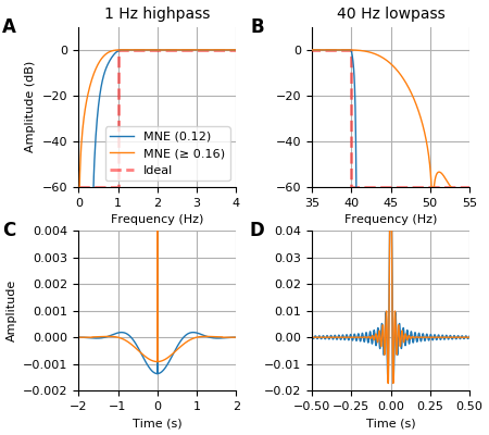
The defaults in MNE 0.12 are slightly different from the defaults in MNE 0.16. For more detailed information regarding these choices, head over to the filtering tutorial on the MNE website.
Here we define a function to design the filters using
scipy.signal.firwin() (0.16) or scipy.signal.firwin2() (0.12).
def design_filter(filter_type, f_p, fir_design, trans_bandwidth,
                  filter_length, fir_window):
    if filter_type == 'highpass':
        h = create_filter(np.ones(100000), sfreq, f_p, None,
                          l_trans_bandwidth=trans_bandwidth,
                          filter_length=filter_length,
                          fir_design=fir_design, fir_window=fir_window)
    else:
        h = create_filter(np.ones(100000), sfreq, None, f_p,
                          h_trans_bandwidth=trans_bandwidth,
                          filter_length=filter_length,
                          fir_design=fir_design, fir_window=fir_window)
    return h
To choose our filters, we plot the frequency response of the filter (in dB). Higher attenuation is good for reducing noise.
However, filters can introduce ripples in the time domain. So, we also plot
the impulse response h of the filter.
def plot_impulse_response(ax, h, label, xlim, ylim):
    dur = 20.
    h_plot = np.zeros((int(dur * sfreq), ))
    start = len(h_plot) // 2 - len(h) // 2
    stop = start + len(h)
    h_plot[start:stop] = h
    t = np.arange(len(h_plot)) / sfreq - dur / 2
    ax.plot(t, h_plot, label=label)
    ax.set(xlim=xlim, ylim=ylim, xlabel='Time (s)',
           ylabel='Amplitude')
Now we plot the frequency response and impulse response for the lowpass and highpass filters in MNE versions 0.12 and 0.16.
fig, axes = plt.subplots(2, 2, figsize=(4.5, 4))

filterlims = dict(highpass=[0, 4.], lowpass=[35, 55])
dblim = [-60, 10]  # for dB plots
f_ps = [1., 40.]  # corner frequencies (Hz)
filter_types = ['highpass', 'lowpass']
xlims = [(-2, 2), (-0.5, 0.5)]
ylims = [(-0.002, 0.004), (-0.02, 0.04)]
fig_num = {0: 'a', 1: 'b', 2: 'c', 3: 'd'}
idx = 0

for ax, f_p, filter_type, xlim, ylim in zip(axes.T, f_ps, filter_types, xlims,
                                            ylims):
    # MNE old defaults
    h = design_filter(filter_type, f_p, 'firwin2', 0.5, '10s', 'hamming')
    lbl = 'MNE (0.12)'
    plot_filter_response(ax[0], h, filterlims[filter_type], label=lbl)
    plot_impulse_response(ax[1], h, lbl, xlim, ylim)

    # MNE new defaults
    h = design_filter(filter_type, f_p, 'firwin', 'auto', 'auto', 'hamming')
    lbl = u'MNE (≥ 0.16)'
    plot_filter_response(ax[0], h, filterlims[filter_type], label=lbl)
    plot_impulse_response(ax[1], h, lbl, xlim, ylim)

    # Ideal gain
    freq = [0, f_p, f_p, sfreq / 2.]
    min_gain = 10 ** (dblim[0] / 20)
    if filter_type == "highpass":
        gain = [min_gain, min_gain, 1, 1]
    else:
        gain = [1, 1, min_gain, min_gain]
    ax[0].plot(freq, 20 * np.log10(gain), 'r--', alpha=0.5,
               linewidth=2, zorder=3, label='Ideal')
    if filter_type == 'highpass':
        ax[0].legend(loc='lower right')
    else:
        ax[0].set(ylabel='')
        ax[1].set(ylabel='')
    ax[0].set(title='%d Hz %s' % (f_p, filter_type))

for ii, (ax, label) in enumerate(zip(axes.ravel(), ['A', 'B', 'C', 'D'])):
    xy = (-0.3, 1) if ii % 2 else (-0.4, 1)
    ax.annotate(label, xy=xy, **annot_kwargs)

fig.tight_layout(pad=0.5, w_pad=2.0, h_pad=0.1)
plt.show()
plt.savefig(op.join('..', 'figures', 'filters.pdf'), bbox_to_inches='tight')
Out:
Setting up high-pass filter at 1 Hz
Filter length of 11000 samples (10.000 sec) selected
Setting up high-pass filter at 1 Hz
l_trans_bandwidth chosen to be 1.0 Hz
Filter length of 3631 samples (3.301 sec) selected
Setting up low-pass filter at 40 Hz
Filter length of 11000 samples (10.000 sec) selected
Setting up low-pass filter at 40 Hz
h_trans_bandwidth chosen to be 10.0 Hz
Filter length of 363 samples (0.330 sec) selected
Total running time of the script: ( 0 minutes 4.507 seconds)