PSD (linear vs log scale)
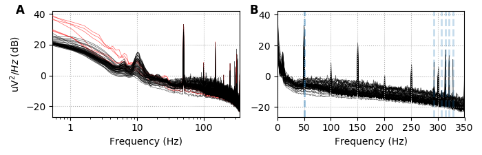
The Power Spectral Density (PSD) plot shows different information for linear vs. log scale. We will demonstrate here how the PSD plot can be used to conveniently spot bad sensors.
import os
import os.path as op
import sys

import matplotlib.pyplot as plt

import mne

sys.path.append(op.join('..', '..', 'processing'))
from library.config import (study_path, map_subjects, annot_kwargs,
                            set_matplotlib_defaults)  # noqa: E402
First some basic configuration as in all scripts
subjects_dir = os.path.join(study_path, 'subjects')

subject_id = 10
run = 2
subject = "sub%03d" % int(subject_id)

fname = op.join(study_path, 'ds117', subject, 'MEG', 'run_%02d_raw.fif' % run)
raw = mne.io.read_raw_fif(fname, preload=True)
Out:
Opening raw data file /tsi/doctorants/data_gramfort/dgw_faces_reproduce/ds117/sub010/MEG/run_02_raw.fif...
    Read a total of 8 projection items:
        mag_ssp_upright.fif : PCA-mags-v1 (1 x 306)  idle
        mag_ssp_upright.fif : PCA-mags-v2 (1 x 306)  idle
        mag_ssp_upright.fif : PCA-mags-v3 (1 x 306)  idle
        mag_ssp_upright.fif : PCA-mags-v4 (1 x 306)  idle
        mag_ssp_upright.fif : PCA-mags-v5 (1 x 306)  idle
        grad_ssp_upright.fif : PCA-grad-v1 (1 x 306)  idle
        grad_ssp_upright.fif : PCA-grad-v2 (1 x 306)  idle
        grad_ssp_upright.fif : PCA-grad-v3 (1 x 306)  idle
    Range : 51700 ... 596199 =     47.000 ...   541.999 secs
Ready.
Current compensation grade : 0
Reading 0 ... 544499  =      0.000 ...   494.999 secs...
Next, we get the list of bad channels
mapping = map_subjects[subject_id]
bads = list()
bad_name = op.join('..', '..', 'processing', 'bads', mapping,
                   'run_%02d_raw_tr.fif_bad' % run)
with open(bad_name) as f:
    for line in f:
        bads.append(line.strip())
and set the EOG/ECG channels appropriately
raw.set_channel_types({'EEG061': 'eog',
                       'EEG062': 'eog',
                       'EEG063': 'ecg',
                       'EEG064': 'misc'})  # EEG064 free floating el.
raw.rename_channels({'EEG061': 'EOG061',
                     'EEG062': 'EOG062',
                     'EEG063': 'ECG063'})

raw.pick_types(eeg=True, meg=False)
MNE also displays the cutoff frequencies of the online filters, but here we remove it from the info and show only the HPI coil frequencies.
raw.info['lowpass'] = None
raw.info['highpass'] = None
raw.info['line_freq'] = None
The line colors for the bad channels will be red.
colors = ['k'] * raw.info['nchan']
for b in bads:
    colors[raw.info['ch_names'].index(b)] = 'r'

# this channel should have been marked bad (subject=14, run=01)
# colors[raw.info['ch_names'].index('EEG024')] = 'g'
First we show the log scale to spot bad sensors.
fig, axes = plt.subplots(1, 2, figsize=(7, 2.25))
set_matplotlib_defaults()
ax = axes[0]
raw.plot_psd(
    average=False, line_alpha=0.6, fmin=0, fmax=350, xscale='log',
    spatial_colors=False, show=False, ax=[ax])
ax.set(xlabel='Frequency (Hz)', title='')
# A little hack fix for matplotlib bug on some systems
for text in fig.axes[0].texts:
    pos = text.get_position()
    if pos[0] <= 0:
        text.set_position([0.1, pos[1]])

for l, c in zip(ax.get_lines(), colors):
    if c == 'r':
        l.set_color(c)
        l.set_zorder(3)
    else:
        l.set_zorder(4)

# Next, the linear scale to check power line frequency

ax = axes[1]
raw.plot_psd(
    average=False, line_alpha=0.6, n_fft=2048, n_overlap=1024, fmin=0,
    fmax=350, xscale='linear', spatial_colors=False, show=False, ax=[ax])
ax.set(xlabel='Frequency (Hz)', ylabel='', title='')
ax.axvline(50., linestyle='--', alpha=0.25, linewidth=2)
ax.axvline(50., linestyle='--', alpha=0.25, linewidth=2)

for ai, (ax, label) in enumerate(zip(axes, 'AB')):
    ax.annotate(label, (-0.15 if ai == 0 else -0.1, 1), **annot_kwargs)

# HPI coils
for freq in [293., 307., 314., 321., 328.]:
    ax.axvline(freq, linestyle='--', alpha=0.25, linewidth=2, zorder=2)

fig.tight_layout()
fig.savefig(op.join('..', 'figures', 'psd.pdf'), bbox_to_inches='tight')
plt.show()
Out:
Effective window size : 1.862 (s)
Effective window size : 1.862 (s)
Total running time of the script: ( 0 minutes 15.697 seconds)