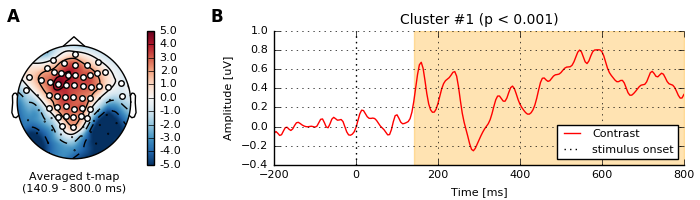
Spatio-temporal sensor-space statistics (EEG)
Run a non-parametric spatio-temporal cluster stats on EEG sensors on the contrast faces vs. scrambled.
import os.path as op
import sys

import numpy as np
from scipy import stats
import matplotlib.pyplot as plt
from mpl_toolkits.axes_grid1 import make_axes_locatable

import mne
from mne.stats import permutation_cluster_1samp_test
from mne.viz import plot_topomap

sys.path.append(op.join('..', '..', 'processing'))
from library.config import (meg_dir, l_freq, exclude_subjects, annot_kwargs,
                            set_matplotlib_defaults, random_state)  # noqa: E402
Read all the data
contrasts = list()

for subject_id in range(1, 20):
    if subject_id in exclude_subjects:
        continue
    subject = "sub%03d" % subject_id
    print("processing subject: %s" % subject)
    data_path = op.join(meg_dir, subject)
    contrast = mne.read_evokeds(op.join(data_path, '%s_highpass-%sHz-ave.fif'
                                        % (subject, l_freq)),
                                condition='contrast')
    contrast.pick_types(meg=False, eeg=True).crop(None, 0.8)
    contrast.apply_baseline((-0.2, 0.0))
    contrasts.append(contrast)

contrast = mne.combine_evoked(contrasts, 'equal')
Out:
processing subject: sub002
Reading /tsi/doctorants/data_gramfort/dgw_faces_reproduce/MEG/sub002/sub002_highpass-NoneHz-ave.fif ...
    Read a total of 1 projection items:
        Average EEG reference (1 x 70) active
    Found the data of interest:
        t =    -200.00 ...    2900.00 ms (contrast)
        0 CTF compensation matrices available
        nave = 155 - aspect type = 100
Projections have already been applied. Setting proj attribute to True.
No baseline correction applied
Applying baseline correction (mode: mean)
processing subject: sub003
Reading /tsi/doctorants/data_gramfort/dgw_faces_reproduce/MEG/sub003/sub003_highpass-NoneHz-ave.fif ...
    Read a total of 1 projection items:
        Average EEG reference (1 x 70) active
    Found the data of interest:
        t =    -200.00 ...    2900.00 ms (contrast)
        0 CTF compensation matrices available
        nave = 146 - aspect type = 100
Projections have already been applied. Setting proj attribute to True.
No baseline correction applied
Applying baseline correction (mode: mean)
processing subject: sub004
Reading /tsi/doctorants/data_gramfort/dgw_faces_reproduce/MEG/sub004/sub004_highpass-NoneHz-ave.fif ...
    Read a total of 1 projection items:
        Average EEG reference (1 x 70) active
    Found the data of interest:
        t =    -200.00 ...    2900.00 ms (contrast)
        0 CTF compensation matrices available
        nave = 139 - aspect type = 100
Projections have already been applied. Setting proj attribute to True.
No baseline correction applied
Applying baseline correction (mode: mean)
processing subject: sub006
Reading /tsi/doctorants/data_gramfort/dgw_faces_reproduce/MEG/sub006/sub006_highpass-NoneHz-ave.fif ...
    Read a total of 1 projection items:
        Average EEG reference (1 x 70) active
    Found the data of interest:
        t =    -200.00 ...    2900.00 ms (contrast)
        0 CTF compensation matrices available
        nave = 108 - aspect type = 100
Projections have already been applied. Setting proj attribute to True.
No baseline correction applied
Applying baseline correction (mode: mean)
processing subject: sub007
Reading /tsi/doctorants/data_gramfort/dgw_faces_reproduce/MEG/sub007/sub007_highpass-NoneHz-ave.fif ...
    Read a total of 1 projection items:
        Average EEG reference (1 x 70) active
    Found the data of interest:
        t =    -200.00 ...    2900.00 ms (contrast)
        0 CTF compensation matrices available
        nave = 193 - aspect type = 100
Projections have already been applied. Setting proj attribute to True.
No baseline correction applied
Applying baseline correction (mode: mean)
processing subject: sub008
Reading /tsi/doctorants/data_gramfort/dgw_faces_reproduce/MEG/sub008/sub008_highpass-NoneHz-ave.fif ...
    Read a total of 1 projection items:
        Average EEG reference (1 x 70) active
    Found the data of interest:
        t =    -200.00 ...    2900.00 ms (contrast)
        0 CTF compensation matrices available
        nave = 127 - aspect type = 100
Projections have already been applied. Setting proj attribute to True.
No baseline correction applied
Applying baseline correction (mode: mean)
processing subject: sub009
Reading /tsi/doctorants/data_gramfort/dgw_faces_reproduce/MEG/sub009/sub009_highpass-NoneHz-ave.fif ...
    Read a total of 1 projection items:
        Average EEG reference (1 x 70) active
    Found the data of interest:
        t =    -200.00 ...    2900.00 ms (contrast)
        0 CTF compensation matrices available
        nave = 89 - aspect type = 100
Projections have already been applied. Setting proj attribute to True.
No baseline correction applied
Applying baseline correction (mode: mean)
processing subject: sub010
Reading /tsi/doctorants/data_gramfort/dgw_faces_reproduce/MEG/sub010/sub010_highpass-NoneHz-ave.fif ...
    Read a total of 1 projection items:
        Average EEG reference (1 x 70) active
    Found the data of interest:
        t =    -200.00 ...    2900.00 ms (contrast)
        0 CTF compensation matrices available
        nave = 115 - aspect type = 100
Projections have already been applied. Setting proj attribute to True.
No baseline correction applied
Applying baseline correction (mode: mean)
processing subject: sub011
Reading /tsi/doctorants/data_gramfort/dgw_faces_reproduce/MEG/sub011/sub011_highpass-NoneHz-ave.fif ...
    Read a total of 1 projection items:
        Average EEG reference (1 x 70) active
    Found the data of interest:
        t =    -200.00 ...    2900.00 ms (contrast)
        0 CTF compensation matrices available
        nave = 113 - aspect type = 100
Projections have already been applied. Setting proj attribute to True.
No baseline correction applied
Applying baseline correction (mode: mean)
processing subject: sub012
Reading /tsi/doctorants/data_gramfort/dgw_faces_reproduce/MEG/sub012/sub012_highpass-NoneHz-ave.fif ...
    Read a total of 1 projection items:
        Average EEG reference (1 x 70) active
    Found the data of interest:
        t =    -200.00 ...    2900.00 ms (contrast)
        0 CTF compensation matrices available
        nave = 116 - aspect type = 100
Projections have already been applied. Setting proj attribute to True.
No baseline correction applied
Applying baseline correction (mode: mean)
processing subject: sub013
Reading /tsi/doctorants/data_gramfort/dgw_faces_reproduce/MEG/sub013/sub013_highpass-NoneHz-ave.fif ...
    Read a total of 1 projection items:
        Average EEG reference (1 x 70) active
    Found the data of interest:
        t =    -200.00 ...    2900.00 ms (contrast)
        0 CTF compensation matrices available
        nave = 120 - aspect type = 100
Projections have already been applied. Setting proj attribute to True.
No baseline correction applied
Applying baseline correction (mode: mean)
processing subject: sub014
Reading /tsi/doctorants/data_gramfort/dgw_faces_reproduce/MEG/sub014/sub014_highpass-NoneHz-ave.fif ...
    Read a total of 1 projection items:
        Average EEG reference (1 x 70) active
    Found the data of interest:
        t =    -200.00 ...    2900.00 ms (contrast)
        0 CTF compensation matrices available
        nave = 116 - aspect type = 100
Projections have already been applied. Setting proj attribute to True.
No baseline correction applied
Applying baseline correction (mode: mean)
processing subject: sub015
Reading /tsi/doctorants/data_gramfort/dgw_faces_reproduce/MEG/sub015/sub015_highpass-NoneHz-ave.fif ...
    Read a total of 1 projection items:
        Average EEG reference (1 x 70) active
    Found the data of interest:
        t =    -200.00 ...    2900.00 ms (contrast)
        0 CTF compensation matrices available
        nave = 60 - aspect type = 100
Projections have already been applied. Setting proj attribute to True.
No baseline correction applied
Applying baseline correction (mode: mean)
processing subject: sub017
Reading /tsi/doctorants/data_gramfort/dgw_faces_reproduce/MEG/sub017/sub017_highpass-NoneHz-ave.fif ...
    Read a total of 1 projection items:
        Average EEG reference (1 x 70) active
    Found the data of interest:
        t =    -200.00 ...    2900.00 ms (contrast)
        0 CTF compensation matrices available
        nave = 89 - aspect type = 100
Projections have already been applied. Setting proj attribute to True.
No baseline correction applied
Applying baseline correction (mode: mean)
processing subject: sub018
Reading /tsi/doctorants/data_gramfort/dgw_faces_reproduce/MEG/sub018/sub018_highpass-NoneHz-ave.fif ...
    Read a total of 1 projection items:
        Average EEG reference (1 x 70) active
    Found the data of interest:
        t =    -200.00 ...    2900.00 ms (contrast)
        0 CTF compensation matrices available
        nave = 135 - aspect type = 100
Projections have already been applied. Setting proj attribute to True.
No baseline correction applied
Applying baseline correction (mode: mean)
processing subject: sub019
Reading /tsi/doctorants/data_gramfort/dgw_faces_reproduce/MEG/sub019/sub019_highpass-NoneHz-ave.fif ...
    Read a total of 1 projection items:
        Average EEG reference (1 x 70) active
    Found the data of interest:
        t =    -200.00 ...    2900.00 ms (contrast)
        0 CTF compensation matrices available
        nave = 138 - aspect type = 100
Projections have already been applied. Setting proj attribute to True.
No baseline correction applied
Applying baseline correction (mode: mean)
Assemble the data and run the cluster stats on channel data
data = np.array([c.data for c in contrasts])

connectivity = None
tail = 0.  # for two sided test

# set cluster threshold
p_thresh = 0.01 / (1 + (tail == 0))
n_samples = len(data)
threshold = -stats.t.ppf(p_thresh, n_samples - 1)
if np.sign(tail) < 0:
    threshold = -threshold

# Make a triangulation between EEG channels locations to
# use as connectivity for cluster level stat
connectivity = mne.channels.find_ch_connectivity(contrast.info, 'eeg')[0]

data = np.transpose(data, (0, 2, 1))  # transpose for clustering

cluster_stats = permutation_cluster_1samp_test(
    data, threshold=threshold, n_jobs=2, verbose=True, tail=1,
    connectivity=connectivity, out_type='indices',
    check_disjoint=True, step_down_p=0.05, seed=random_state)

T_obs, clusters, p_values, _ = cluster_stats
good_cluster_inds = np.where(p_values < 0.05)[0]

print("Good clusters: %s" % good_cluster_inds)
Out:
Could not find a connectivity matrix for the data. Computing connectivity based on Delaunay triangulations.
-- number of connected vertices : 70
stat_fun(H1): min=-9.714884 max=12.075012
No disjoint connectivity sets found
Running initial clustering
Found 8 clusters
Permuting 1023 times...
Computing cluster p-values
Step-down-in-jumps iteration #1 found 1 cluster to exclude from subsequent iterations
Permuting 1023 times...
Computing cluster p-values
Step-down-in-jumps iteration #2 found 0 additional clusters to exclude from subsequent iterations
Done.
Good clusters: [7]
Visualize the spatio-temporal clusters
set_matplotlib_defaults()
times = contrast.times * 1e3
colors = 'r', 'steelblue'
linestyles = '-', '--'

pos = mne.find_layout(contrast.info).pos

T_obs_max = 5.
T_obs_min = -T_obs_max

# loop over significant clusters
for i_clu, clu_idx in enumerate(good_cluster_inds):

    # unpack cluster information, get unique indices
    time_inds, space_inds = np.squeeze(clusters[clu_idx])
    ch_inds = np.unique(space_inds)
    time_inds = np.unique(time_inds)

    # get topography for T0 stat
    T_obs_map = T_obs[time_inds, ...].mean(axis=0)

    # get signals at significant sensors
    signals = data[..., ch_inds].mean(axis=-1)
    sig_times = times[time_inds]

    # create spatial mask
    mask = np.zeros((T_obs_map.shape[0], 1), dtype=bool)
    mask[ch_inds, :] = True

    # initialize figure
    fig, ax_topo = plt.subplots(1, 1, figsize=(7, 2.))

    # plot average test statistic and mark significant sensors
    image, _ = plot_topomap(T_obs_map, pos, mask=mask, axes=ax_topo,
                            vmin=T_obs_min, vmax=T_obs_max,
                            show=False)

    # advanced matplotlib for showing image with figure and colorbar
    # in one plot
    divider = make_axes_locatable(ax_topo)

    # add axes for colorbar
    ax_colorbar = divider.append_axes('right', size='5%', pad=0.05)
    plt.colorbar(image, cax=ax_colorbar, format='%0.1f')
    ax_topo.set_xlabel('Averaged t-map\n({:0.1f} - {:0.1f} ms)'.format(
        *sig_times[[0, -1]]
    ))
    ax_topo.annotate(chr(65 + 2 * i_clu), (0.1, 1.1), **annot_kwargs)

    # add new axis for time courses and plot time courses
    ax_signals = divider.append_axes('right', size='300%', pad=1.2)
    for signal, name, col, ls in zip(signals, ['Contrast'], colors,
                                     linestyles):
        ax_signals.plot(times, signal * 1e6, color=col,
                        linestyle=ls, label=name)

    # add information
    ax_signals.axvline(0, color='k', linestyle=':', label='stimulus onset')
    ax_signals.set_xlim([times[0], times[-1]])
    ax_signals.set_xlabel('Time [ms]')
    ax_signals.set_ylabel('Amplitude [uV]')

    # plot significant time range
    ymin, ymax = ax_signals.get_ylim()
    ax_signals.fill_betweenx((ymin, ymax), sig_times[0], sig_times[-1],
                             color='orange', alpha=0.3)
    ax_signals.legend(loc='lower right')
    title = 'Cluster #{0} (p < {1:0.3f})'.format(i_clu + 1, p_values[clu_idx])
    ax_signals.set(ylim=[ymin, ymax], title=title)
    ax_signals.annotate(chr(65 + 2 * i_clu + 1), (-0.125, 1.1), **annot_kwargs)

    # clean up viz
    fig.tight_layout(pad=0.5, w_pad=0)
    fig.subplots_adjust(bottom=.05)
    plt.savefig(op.join('..', 'figures',
                        'spatiotemporal_stats_cluster_highpass-%sHz-%02d.pdf'
                        % (l_freq, i_clu)))
    plt.show()
Total running time of the script: ( 0 minutes 15.428 seconds)