Decoding (ML) across time (MEG)¶

A sliding estimator fits a logistic regression model for every time point. In this example, we contrast the condition ‘famous’ vs ‘scrambled’ and ‘famous’ vs ‘unfamiliar’ using this approach. The end result is an averaging effect across sensors. The contrast across different sensors are combined into a single plot.

Analysis script: Sliding estimator

Let us first import the necessary libraries

import os
import os.path as op
import sys

import numpy as np
import matplotlib.pyplot as plt
from scipy.io import loadmat
from scipy.stats import sem

sys.path.append(op.join('..', '..', 'processing'))
from library.config import (meg_dir, l_freq, annot_kwargs, tmax,
                            set_matplotlib_defaults)  # noqa: E402

Now we loop over subjects to load the scores

a_vs_bs = ['face_vs_scrambled', 'famous_vs_unfamiliar']
scores = {'face_vs_scrambled': list(), 'famous_vs_unfamiliar': list()}
for subject_id in range(1, 20):
    subject = "sub%03d" % subject_id
    data_path = os.path.join(meg_dir, subject)

    # Load the scores for the subject
    for a_vs_b in a_vs_bs:
        fname_td = os.path.join(data_path, '%s_highpass-%sHz-td-auc-%s.mat'
                                % (subject, l_freq, a_vs_b))
        mat = loadmat(fname_td)
        scores[a_vs_b].append(mat['scores'][0])

… and average them

times = mat['times'][0]
mean_scores, sem_scores = dict(), dict()
for a_vs_b in a_vs_bs:
    mean_scores[a_vs_b] = np.mean(scores[a_vs_b], axis=0)
    sem_scores[a_vs_b] = sem(scores[a_vs_b])

Let’s plot the mean AUC score across subjects

set_matplotlib_defaults()
colors = ['b', 'g']
fig, ax = plt.subplots(1, figsize=(3.3, 2.5))
for c, a_vs_b in zip(colors, a_vs_bs):
    ax.plot(times, mean_scores[a_vs_b], c, label=a_vs_b.replace('_', ' '))
    ax.set(xlabel='Time (s)', ylabel='Area under curve (AUC)')
    ax.fill_between(times, mean_scores[a_vs_b] - sem_scores[a_vs_b],
                    mean_scores[a_vs_b] + sem_scores[a_vs_b],
                    color=c, alpha=0.33, edgecolor='none')
ax.axhline(0.5, color='k', linestyle='--', label='Chance level')
ax.axvline(0.0, color='k', linestyle='--')
ax.legend()
ax.set(xlim=[-0.2, tmax])
ax.annotate('B', (-0.15, 1), **annot_kwargs)
fig.tight_layout(pad=0.5)
fig.savefig(op.join('..', 'figures', 'time_decoding_highpass-%sHz.pdf'
                    % (l_freq,)), bbox_to_inches='tight')
plt.show()

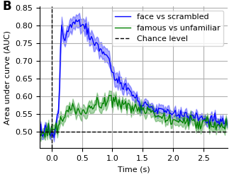
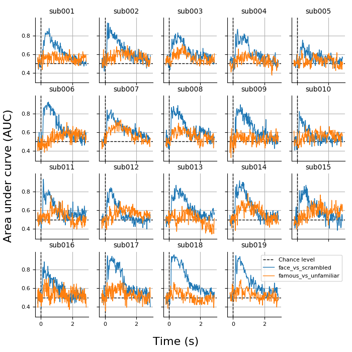
../../_images/sphx_glr_plot_sliding_estimator_001.png

It seems that ‘famous’ vs ‘unfamiliar’ gives much noisier time course of decoding scores than ‘faces’ vs ‘scrambled’. To verify that this is not due to bad subjects:

fig, axes = plt.subplots(4, 5, sharex=True, sharey=True,
                         figsize=(7, 7))
axes = axes.ravel()
for idx in range(19):
    axes[idx].axhline(0.5, color='k', linestyle='--', label='Chance level')
    axes[idx].axvline(0.0, color='k', linestyle='--')
    for a_vs_b in a_vs_bs:
        axes[idx].plot(times, scores[a_vs_b][idx], label=a_vs_b)
        axes[idx].set_title('sub%03d' % (idx + 1))

axes[-1].axis('off')
axes[-2].legend(bbox_to_anchor=(2.2, 0.75), loc='center right')
fig.text(0.5, 0.02, 'Time (s)', ha='center', fontsize=16)
fig.text(0.01, 0.5, 'Area under curve (AUC)', va='center',
         rotation='vertical', fontsize=16)
fig.subplots_adjust(bottom=0.1, left=0.1, right=0.98, top=0.95)
plt.show()

../../_images/sphx_glr_plot_sliding_estimator_002.png

Total running time of the script: ( 0 minutes 2.530 seconds)

Gallery generated by Sphinx-Gallery