Note
Go to the end to download the full example code.
Corrupt known signal with point spread#
The aim of this tutorial is to demonstrate how to put a known signal at a
desired location(s) in a mne.SourceEstimate and then corrupt the
signal with point-spread by applying a forward and inverse solution.
# License: BSD-3-Clause
# Copyright the MNE-Python contributors.
import numpy as np

import mne
from mne.datasets import sample
from mne.minimum_norm import apply_inverse, read_inverse_operator
from mne.simulation import simulate_evoked, simulate_stc
First, we set some parameters.
seed = 42

# parameters for inverse method
method = "sLORETA"
snr = 3.0
lambda2 = 1.0 / snr**2

# signal simulation parameters
# do not add extra noise to the known signals
nave = np.inf
T = 100
times = np.linspace(0, 1, T)
dt = times[1] - times[0]

# Paths to MEG data
data_path = sample.data_path()
subjects_dir = data_path / "subjects"
fname_fwd = data_path / "MEG" / "sample" / "sample_audvis-meg-oct-6-fwd.fif"
fname_inv = data_path / "MEG" / "sample" / "sample_audvis-meg-oct-6-meg-fixed-inv.fif"
fname_evoked = data_path / "MEG" / "sample" / "sample_audvis-ave.fif"
Load the MEG data#
fwd = mne.read_forward_solution(fname_fwd)
fwd = mne.convert_forward_solution(fwd, force_fixed=True, surf_ori=True, use_cps=False)
fwd["info"]["bads"] = []
inv_op = read_inverse_operator(fname_inv)

raw = mne.io.read_raw_fif(data_path / "MEG" / "sample" / "sample_audvis_raw.fif")
raw.info["bads"] = []
raw.set_eeg_reference(projection=True)
events = mne.find_events(raw)
event_id = {"Auditory/Left": 1, "Auditory/Right": 2}
epochs = mne.Epochs(raw, events, event_id, baseline=(None, 0), preload=True)
evoked = epochs.average()

labels = mne.read_labels_from_annot("sample", subjects_dir=subjects_dir)
label_names = [label.name for label in labels]
n_labels = len(labels)
Reading forward solution from /home/circleci/mne_data/MNE-sample-data/MEG/sample/sample_audvis-meg-oct-6-fwd.fif...
    Reading a source space...
    Computing patch statistics...
    Patch information added...
    Distance information added...
    [done]
    Reading a source space...
    Computing patch statistics...
    Patch information added...
    Distance information added...
    [done]
    2 source spaces read
    Desired named matrix (kind = 3523) not available
    Read MEG forward solution (7498 sources, 306 channels, free orientations)
    Source spaces transformed to the forward solution coordinate frame
    Changing to fixed-orientation forward solution with surface-based source orientations...
    [done]
Reading inverse operator decomposition from /home/circleci/mne_data/MNE-sample-data/MEG/sample/sample_audvis-meg-oct-6-meg-fixed-inv.fif...
    Reading inverse operator info...
    [done]
    Reading inverse operator decomposition...
    [done]
    305 x 305 full covariance (kind = 1) found.
    Read a total of 4 projection items:
        PCA-v1 (1 x 10²) active
        PCA-v2 (1 x 10²) active
        PCA-v3 (1 x 10²) active
        Average EEG reference (1 x 60) active
    Noise covariance matrix read.
    7498 x 7498 diagonal covariance (kind = 2) found.
    Source covariance matrix read.
    Did not find the desired covariance matrix (kind = 6)
    7498 x 7498 diagonal covariance (kind = 5) found.
    Depth priors read.
    Did not find the desired covariance matrix (kind = 3)
    Reading a source space...
    Computing patch statistics...
    Patch information added...
    Distance information added...
    [done]
    Reading a source space...
    Computing patch statistics...
    Patch information added...
    Distance information added...
    [done]
    2 source spaces read
    Read a total of 4 projection items:
        PCA-v1 (1 x 10²) active
        PCA-v2 (1 x 10²) active
        PCA-v3 (1 x 10²) active
        Average EEG reference (1 x 60) active
    Source spaces transformed to the inverse solution coordinate frame
Opening raw data file /home/circleci/mne_data/MNE-sample-data/MEG/sample/sample_audvis_raw.fif...
    Read a total of 3 projection items:
        PCA-v1 (1 x 10²)  idle
        PCA-v2 (1 x 10²)  idle
        PCA-v3 (1 x 10²)  idle
    Range : 25800 ... 192599 =     42.956 ...   320.670 secs
Ready.
EEG channel type selected for re-referencing
Adding average EEG reference projection.
1 projection items deactivated
320 events found on stim channel STI 014
Event IDs: [ 1  2  3  4  5 32]
Not setting metadata
145 matching events found
Setting baseline interval to [-0.19979521315838786, 0.0] s
Applying baseline correction (mode: mean)
Created an SSP operator (subspace dimension = 4)
4 projection items activated
Loading data for 145 events and 421 original time points ...
0 bad epochs dropped
Reading labels from parcellation...
   read 34 labels from /home/circleci/mne_data/MNE-sample-data/subjects/sample/label/lh.aparc.annot
   read 34 labels from /home/circleci/mne_data/MNE-sample-data/subjects/sample/label/rh.aparc.annot
Estimate the background noise covariance from the baseline period#
cov = mne.compute_covariance(epochs, tmin=None, tmax=0.0)
    Created an SSP operator (subspace dimension = 4)
    Setting small MEG eigenvalues to zero (without PCA)
    Setting small EEG eigenvalues to zero (without PCA)
Reducing data rank from 366 -> 362
Estimating covariance using EMPIRICAL
Done.
Number of samples used : 17545
[done]
Generate sinusoids in two spatially distant labels#
# The known signal is all zero-s off of the two labels of interest
signal = np.zeros((n_labels, T))
idx = label_names.index("inferiorparietal-lh")
signal[idx, :] = 1e-7 * np.sin(5 * 2 * np.pi * times)
idx = label_names.index("rostralmiddlefrontal-rh")
signal[idx, :] = 1e-7 * np.sin(7 * 2 * np.pi * times)
Find the center vertices in source space of each label#
We want the known signal in each label to only be active at the center. We create a mask for each label that is 1 at the center vertex and 0 at all other vertices in the label. This mask is then used when simulating source-space data.
hemi_to_ind = {"lh": 0, "rh": 1}
for i, label in enumerate(labels):
    # The `center_of_mass` function needs labels to have values.
    labels[i].values.fill(1.0)

    # Restrict the eligible vertices to be those on the surface under
    # consideration and within the label.
    surf_vertices = fwd["src"][hemi_to_ind[label.hemi]]["vertno"]
    restrict_verts = np.intersect1d(surf_vertices, label.vertices)
    com = labels[i].center_of_mass(
        subjects_dir=subjects_dir, restrict_vertices=restrict_verts, surf="white"
    )

    # Convert the center of vertex index from surface vertex list to Label's
    # vertex list.
    cent_idx = np.where(label.vertices == com)[0][0]

    # Create a mask with 1 at center vertex and zeros elsewhere.
    labels[i].values.fill(0.0)
    labels[i].values[cent_idx] = 1.0

    # Print some useful information about this vertex and label
    if "transversetemporal" in label.name:
        dist, _ = label.distances_to_outside(subjects_dir=subjects_dir)
        dist = dist[cent_idx]
        area = label.compute_area(subjects_dir=subjects_dir)
        # convert to equivalent circular radius
        r = np.sqrt(area / np.pi)
        print(
            f"{label.name} COM vertex is {dist * 1e3:0.1f} mm from edge "
            f"(label area equivalent to a circle with r={r * 1e3:0.1f} mm)"
        )
    Triangle neighbors and vertex normals...
transversetemporal-lh COM vertex is 7.5 mm from edge (label area equivalent to a circle with r=11.5 mm)
    Triangle neighbors and vertex normals...
transversetemporal-rh COM vertex is 6.8 mm from edge (label area equivalent to a circle with r=10.8 mm)
Create source-space data with known signals#
Put known signals onto surface vertices using the array of signals and the label masks (stored in labels[i].values).
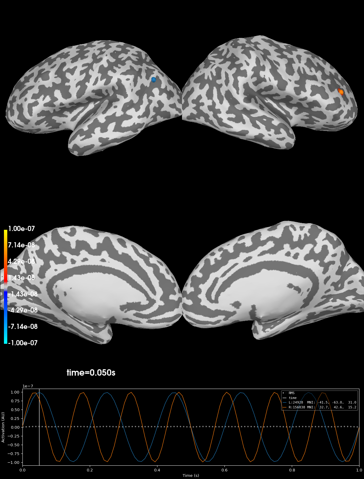
Plot original signals#
Note that the original signals are highly concentrated (point) sources.
kwargs = dict(
    subjects_dir=subjects_dir,
    hemi="split",
    smoothing_steps=4,
    time_unit="s",
    initial_time=0.05,
    size=1200,
    views=["lat", "med"],
)
clim = dict(kind="value", pos_lims=[1e-9, 1e-8, 1e-7])
brain_gen = stc_gen.plot(clim=clim, **kwargs)
Simulate sensor-space signals#
Use the forward solution and add Gaussian noise to simulate sensor-space
(evoked) data from the known source-space signals. The amount of noise is
controlled by nave (higher values imply less noise).
evoked_gen = simulate_evoked(fwd, stc_gen, evoked.info, cov, nave, random_state=seed)

# Map the simulated sensor-space data to source-space using the inverse
# operator.
stc_inv = apply_inverse(evoked_gen, inv_op, lambda2, method=method)
Projecting source estimate to sensor space...
[done]
4 projection items deactivated
Created an SSP operator (subspace dimension = 3)
4 projection items activated
SSP projectors applied...
Preparing the inverse operator for use...
    Scaled noise and source covariance from nave = 1 to nave = 1
    Created the regularized inverter
    Created an SSP operator (subspace dimension = 3)
    Created the whitener using a noise covariance matrix with rank 302 (3 small eigenvalues omitted)
    Computing noise-normalization factors (sLORETA)...
[done]
Applying inverse operator to ""...
    Picked 305 channels from the data
    Computing inverse...
    Eigenleads need to be weighted ...
    Computing residual...
    Explained  99.7% variance
    sLORETA...
[done]
Plot the point-spread of corrupted signal#
Notice that after applying the forward- and inverse-operators to the known point sources that the point sources have spread across the source-space. This spread is due to the minimum norm solution so that the signal leaks to nearby vertices with similar orientations so that signal ends up crossing the sulci and gyri.
brain_inv = stc_inv.plot(**kwargs)
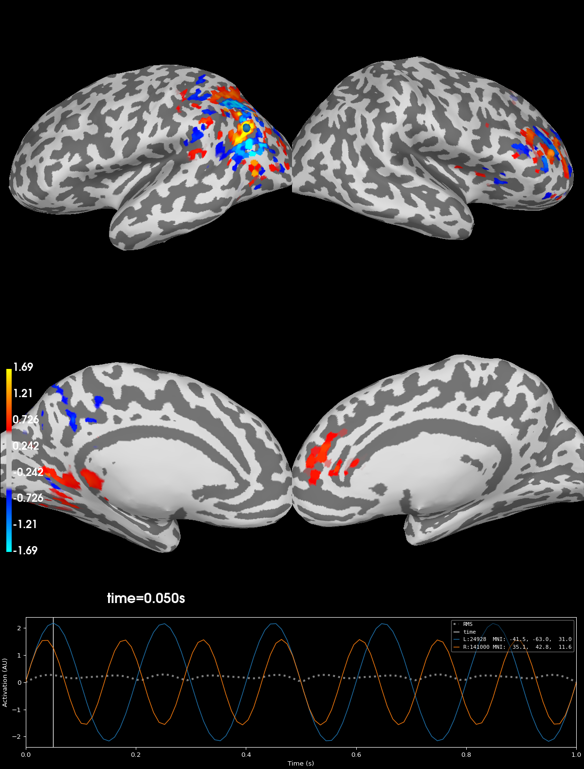
Using control points [0.45968308 0.57021267 1.69354621]
Exercises#
Change the
methodparameter to either'dSPM'or'MNE'to explore the effect of the inverse method.Try setting
evoked_snrto a small, finite value, e.g. 3., to see the effect of noise.
Total running time of the script: (0 minutes 22.540 seconds)
Estimated memory usage: 659 MB